Confounding Variables in Disease Prediction
Accounting for confounding factors in machine learning disease prediction
The healthcare domain is going through profound changes in recent years. The popularity and advancements around machine learning and big data analysis techniques have contributed a lot to one of the major shifts that we are currently witnessing.
The shift from “one size fits all” generic treatments and medications to personalized healthcare and even individualized healthcare.
At DayTwo, we constantly utilize machine learning together with our huge Microbiome dataset to unfold hidden links between the gut bacteria and various diseases in order to advance personalized predictive healthcare.
In this article, we will address the case of disease prediction.
What is disease prediction?
Overall, disease prediction can be divided into four main categories:
- Diagnostics — the ability to predict the presence of a disease.
- Prognostics — the ability to predict a disease outcome and progression.
- Risk — the ability to predict the probability of someone developing a disease in the near future.
- Responders vs Non-Responders — the ability to predict response to treatment or medication.
All methods utilize machine/deep learning as their main tool for creating a predictive model, but each category defines the problem a little bit different.

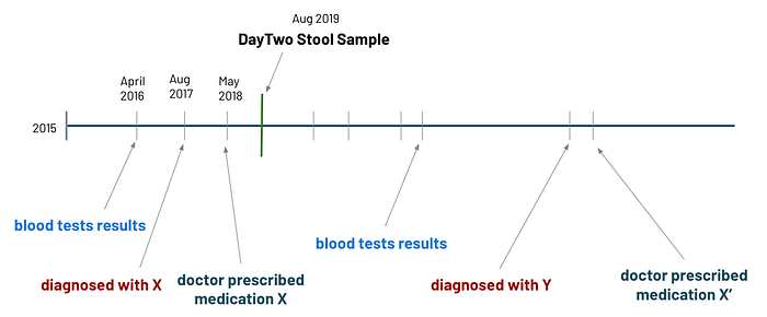
For example, at DayTwo, we use the gut bacteria composition to predict diseases, so in diagnostics, we predict the presence of the disease X by training a machine learning model using all the users who were diagnosed with X before their stool sample day. Whereas in risk prediction, we use all the users who were diagnosed with disease X after they gave their stool samples.
Case Study: Predicting NAFLD using the Gut Microbiome
Let’s consider a case where we have already trained a binary classification machine learning model that can predict whether someone has NAFLD (non-alcoholic fatty liver disease) or not, which we measured on an external test set and received AUC=0.85
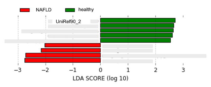
After training the model and applying standard explainability methods, we received a list of the top contributing factors, where each factor was assigned with an effect size score (this can be done with SHAP or any other explainability method).

Calculating Genes and Pathways Effect Size
It is not uncommon that in some cases you need to calculate the effect size of some treatment (a.k.a ATE - average treatment effect). In our case, for simplicity, we consider a treatment to be an increase in the levels of one of the genes.
For example, we analyze the case where we treat NAFLD patients by increasing their gene uniref_90_2 levels to above the population median.
Now, our goal is to measure how increasing the gene levels above this threshold affects NAFLD patients.
Inverse Propensity Weighting
Since we’re working with observational data, and we didn’t run a Randomized Controlled Trial (RCT), we cannot just look at the difference in the disease outcome between the two groups, because the treated and the non-treated groups potentially have very different set of attributes.
A common problem when using observational data is that subjects are not randomly assigned to one of the treatments.
The idea behind IPW is to reweigh each individual in each treatment group to estimate the potential outcome if all subjects in the population were assigned either treatment.
Steps to compute the Estimated Effect Size
1. Computing a propensity score for each individual
Training a logistic regression model using all the potential confounders as features to predict the treatment (in our case the treatment is defined as having gene x above the threshold).
Then, Computing the propensity score for each individual — this score equals the probability of an individual being assigned to treatment (i.e. having gene x above the threshold) given their baseline characteristics.
2. Features weighting
Weighting each individual by the inverse probability of receiving his actual treatment. Weights are calculated for each individual as 1/propensity-score for the exposed group (T=1) and 1–(1/propensity-score) for the unexposed group (T=0).
3. Adding weights to the model
Adding the computed weights to the propensity-score model to generate assignment to treatment - independent from all other features. At this point, we can verify that our weighted model is not able to predict the treatment (AUC=±0.5).

4. Validating features balance
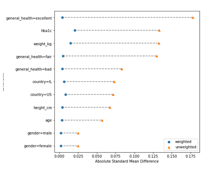
Checking the balance of the features between the two treatment groups by assessing the standardized differences of baseline characteristics included in the propensity score model before and after weighting.

4. Calculating the Estimated Causal Effect
First, estimating the balance outcome using Horvitz–Thompson estimator (on both outcomes). Then, calculate their difference to get the estimated causal effect.


If you’d like to hear more about the latest and greatest we’ve been working on, don’t hesitate to contact me.
